There is another set of values,
the canonical_efficiency_factors, that
are used to evaluate a design but which
has not yet been discussed. Let ![]() be the number of units
receiving treatment
be the number of units
receiving treatment ![]() (this is the general diagonal element of
(this is the general diagonal element of ![]() ) and let
) and let ![]() be the diagonal matrix with
the
be the diagonal matrix with
the ![]() along the diagonal. The canonical efficiency
factors
along the diagonal. The canonical efficiency
factors
In the incomplete block design, the variance of the estimator of
![]() is equal to
is equal to
![]() , while the
variance in a completely randomized design with the same replication
is
, while the
variance in a completely randomized design with the same replication
is
![]() , where the two values of
, where the two values of ![]() are
the variances per plot in the incomplete block design and the
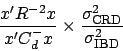
completely randomized design respectively. Therefore the relative
efficiency is
are
the variances per plot in the incomplete block design and the
completely randomized design respectively. Therefore the relative
efficiency is

Since ![]() is symmetric, it can orthogonally diagonalized. The
contrast
is symmetric, it can orthogonally diagonalized. The
contrast ![]() is called a basic contrast if
is called a basic contrast if ![]() for
an eigenvector
for
an eigenvector ![]() of
of ![]() which is not a multiple of
which is not a multiple of ![]() , where
, where
![]() is the all-
is the all-![]() vector. The basic contrasts span the space of
all treatment contrasts; moreover, if
vector. The basic contrasts span the space of
all treatment contrasts; moreover, if ![]() is orthogonal to
is orthogonal to ![]() then the estimators of
then the estimators of ![]() and
and ![]() are
uncorrelated (and independent if the errors are normally distributed).
are
uncorrelated (and independent if the errors are normally distributed).
Each efficiency factor lies between 0 and 1;
at the extremes are contrasts that cannot be estimated (efficiency
factor ![]() ) and contrasts that are
estimated just as well as in an unblocked design with the same
) and contrasts that are
estimated just as well as in an unblocked design with the same
![]() (efficiency factor
(efficiency factor ![]() ).
Thus
).
Thus ![]() is the proportion of information lost to blocking
when estimating a corresponding basic contrast (or any contrast in its
eigenspace);
is the proportion of information lost to blocking
when estimating a corresponding basic contrast (or any contrast in its
eigenspace); ![]() is the proportion of information retained.
Design
is the proportion of information retained.
Design ![]() is disconnected if and only if
is disconnected if and only if ![]() .
.
The comparison to a completely randomized design
with the same replication
numbers is the key concept here.
Efficiency factors evaluate design ![]() over the
universe of all designs with
the same replications
over the
universe of all designs with
the same replications
![]() as
as ![]() ,
constraining the earlier discussed reference universe of competitors
with the given
,
constraining the earlier discussed reference universe of competitors
with the given ![]() and block size distribution.
This constrained universe of comparison is typically justified as
follows: the replication numbers have been purposefully chosen (and thus fixed)
to reflect relative interest in the treatments, or the replication
numbers are forced by the availablity of the material (for example,
scarce amounts of seed of new varieties but plenty of the control
varieties),
so the task is to determine a best (in whatever sense) design within
those constraints. The idealized best (in every sense) is
the completely randomized design (no blocking) so long as this
does not increase the variance per plot. Though experimental
material at hand has forced blocking, the unobtainable CRD can still
be used as a fixed basis for comparison.
and block size distribution.
This constrained universe of comparison is typically justified as
follows: the replication numbers have been purposefully chosen (and thus fixed)
to reflect relative interest in the treatments, or the replication
numbers are forced by the availablity of the material (for example,
scarce amounts of seed of new varieties but plenty of the control
varieties),
so the task is to determine a best (in whatever sense) design within
those constraints. The idealized best (in every sense) is
the completely randomized design (no blocking) so long as this
does not increase the variance per plot. Though experimental
material at hand has forced blocking, the unobtainable CRD can still
be used as a fixed basis for comparison.
Variances of contrasts estimated with a CRD exactly mirror the
selected sample sizes. If the replication numbers are intended
to reflect relative interest in treatments, then a reasonable design
goal is to find ![]() for which variances of all contrast estimators
enjoy the same relative magnitudes as in the CRD. This is exactly
the property of efficiency balance: design
for which variances of all contrast estimators
enjoy the same relative magnitudes as in the CRD. This is exactly
the property of efficiency balance: design ![]() is
efficiency balanced if its canonical efficiency factors are all equal:
is
efficiency balanced if its canonical efficiency factors are all equal:
![]() .
.
For equal block sizes ![]() (
(![]() ), the
only equireplicate, binary, efficiency balanced designs are the BIBDs.
Unfortunately, an unequally replicated design cannot be efficiency balanced
if the block sizes are constant and it is binary. Thus in many
instances the best hope is to approximate the relative interest
intended by the choice of sample sizes. Approximating efficiency
balance (seeking small dispersion in the efficiency factors) will
then be a design goal, typically in conjunction with seeking a high
overall efficiency factor as measured through one or more summary
functions of the canonical efficiency factors. The harmonic mean of the
canonical efficiency factors (see below) is often called
``the'' efficiency factor of a design; if the value is 0.87, for
instance, then use of blocks has resulted in an overall 13%
loss of information.
), the
only equireplicate, binary, efficiency balanced designs are the BIBDs.
Unfortunately, an unequally replicated design cannot be efficiency balanced
if the block sizes are constant and it is binary. Thus in many
instances the best hope is to approximate the relative interest
intended by the choice of sample sizes. Approximating efficiency
balance (seeking small dispersion in the efficiency factors) will
then be a design goal, typically in conjunction with seeking a high
overall efficiency factor as measured through one or more summary
functions of the canonical efficiency factors. The harmonic mean of the
canonical efficiency factors (see below) is often called
``the'' efficiency factor of a design; if the value is 0.87, for
instance, then use of blocks has resulted in an overall 13%
loss of information.
For an equireplicate design (all ![]() are equal--to
are equal--to ![]() say)
the canonical efficiency factors are just 1/
say)
the canonical efficiency factors are just 1/![]() times the inverses
of the canonical variances; some statisticians consider them a more
interpretable alternative to the canonical variances in this case.
If all the efficiency factors are 1, the design is
fully efficient, a property achieved
in the equiblocksize case (with
times the inverses
of the canonical variances; some statisticians consider them a more
interpretable alternative to the canonical variances in this case.
If all the efficiency factors are 1, the design is
fully efficient, a property achieved
in the equiblocksize case (with ![]() ) only by complete block
designs. Consequently, efficiency factors for equireplicate designs
can also be interpreted as
summarizing the loss of information when using incomplete blocks
(block sizes smaller than
) only by complete block
designs. Consequently, efficiency factors for equireplicate designs
can also be interpreted as
summarizing the loss of information when using incomplete blocks
(block sizes smaller than ![]() ) rather than complete blocks.
) rather than complete blocks.
The external representation contains the following commonly
used
summaries_of_efficiency_factors. In terms of these
measures, an optimal design is one which maximizes the value.
Each summary measure induces a design ordering which is identical to
that for one of the optimality_criteria above, based on the
canonical variances, provided the set
of competing designs is restricted to be equireplicate. More generally, these
measures should only be used to compare designs with the
same replication numbers.
![]()
This is the harmonic mean of the efficiency factors.
Equivalent to (produces the same design ordering as) ![]() in the
equireplicate case.
in the
equireplicate case.
![]()
This is the geometric mean of the efficiency
factors. Equivalent to (produces the same design ordering as) ![]() in the equireplicate case.
in the equireplicate case.
The smallest efficiency factor (![]() ). Equivalent to
). Equivalent to ![]() in the
equireplicate case.
in the
equireplicate case.
The Introduction gives an example of a block design which is called the
Fano plane. It is a BIBD for ![]() treatments in
treatments in ![]() blocks of size
blocks of size ![]() .
As with any BIBD, it is pairwise_balanced,
variance_balanced, and efficiency_balanced, and
it is optimal with respect to all of the optimality_criteria
over its entire reference universe. Here are all of the
statistical_properties, that have been discussed so far, for
this example:
.
As with any BIBD, it is pairwise_balanced,
variance_balanced, and efficiency_balanced, and
it is optimal with respect to all of the optimality_criteria
over its entire reference universe. Here are all of the
statistical_properties, that have been discussed so far, for
this example:
<statistical_properties precision="9">
    <canonical_variances no_distinct="1" ordered="true">
        <value multiplicity="6"><d>0.428571429</d></value>
    </canonical_variances>
    <pairwise_variances>
        <function_on_ksubsets_of_indices domain_base="points" k="2" n="7"
         ordered="true">
            <map>
                <preimage>
                    <entire_domain>
                    </entire_domain>
                </preimage>
                <image><d>0.857142857</d></image>
            </map>
        </function_on_ksubsets_of_indices>
    </pairwise_variances>
    <optimality_criteria>
        <phi_0>
            <value><d>-5.08378716</d></value>
            <absolute_efficiency><z>1</z></absolute_efficiency>
            <calculated_efficiency><z>1</z></calculated_efficiency>
        </phi_0>
        <phi_1>
            <value><d>0.428571429</d></value>
            <absolute_efficiency><z>1</z></absolute_efficiency>
            <calculated_efficiency><z>1</z></calculated_efficiency>
        </phi_1>
        <phi_2>
            <value><d>0.183673469</d></value>
            <absolute_efficiency><z>1</z></absolute_efficiency>
            <calculated_efficiency><z>1</z></calculated_efficiency>
        </phi_2>
        <maximum_pairwise_variances>
            <value><d>0.857142857</d></value>
            <absolute_efficiency><z>1</z></absolute_efficiency>
            <calculated_efficiency><z>1</z></calculated_efficiency>
        </maximum_pairwise_variances>
        <E_criteria>
            <E_value index="1">
                <value><d>0.428571429</d></value>
                <absolute_efficiency><z>1</z></absolute_efficiency>
                <calculated_efficiency><z>1</z></calculated_efficiency>
            </E_value>
            <E_value index="2">
                <value><d>0.857142857</d></value>
                <absolute_efficiency><z>1</z></absolute_efficiency>
                <calculated_efficiency><z>1</z></calculated_efficiency>
            </E_value>
            <E_value index="3">
                <value><d>1.28571429</d></value>
                <absolute_efficiency><z>1</z></absolute_efficiency>
                <calculated_efficiency><z>1</z></calculated_efficiency>
            </E_value>
            <E_value index="4">
                <value><d>1.71428571</d></value>
                <absolute_efficiency><z>1</z></absolute_efficiency>
                <calculated_efficiency><z>1</z></calculated_efficiency>
            </E_value>
            <E_value index="5">
                <value><d>2.14285714</d></value>
                <absolute_efficiency><z>1</z></absolute_efficiency>
                <calculated_efficiency><z>1</z></calculated_efficiency>
            </E_value>
            <E_value index="6">
                <value><d>2.57142857</d></value>
                <absolute_efficiency><z>1</z></absolute_efficiency>
                <calculated_efficiency><z>1</z></calculated_efficiency>
            </E_value>
        </E_criteria>
    </optimality_criteria>
    <other_ordering_criteria>
        <trace_of_square_of_C>
            <value><d>32.6666667</d></value>
            <absolute_comparison><z>1</z></absolute_comparison>
            <calculated_comparison><z>1</z></calculated_comparison>
        </trace_of_square_of_C>
        <max_min_ratio_canonical_variances>
            <value><d>1.0</d></value>
            <absolute_comparison><z>1</z></absolute_comparison>
            <calculated_comparison><z>1</z></calculated_comparison>
        </max_min_ratio_canonical_variances>
        <max_min_ratio_pairwise_variances>
            <value><d>1.0</d></value>
            <absolute_comparison><z>1</z></absolute_comparison>
            <calculated_comparison><z>1</z></calculated_comparison>
        </max_min_ratio_pairwise_variances>
        <no_distinct_canonical_variances>
            <value><z>1</z></value>
            <absolute_comparison><z>1</z></absolute_comparison>
            <calculated_comparison><z>1</z></calculated_comparison>
        </no_distinct_canonical_variances>
        <no_distinct_pairwise_variances>
            <value><z>1</z></value>
            <absolute_comparison><z>1</z></absolute_comparison>
            <calculated_comparison><z>1</z></calculated_comparison>
        </no_distinct_pairwise_variances>
    </other_ordering_criteria>
    <canonical_efficiency_factors no_distinct="1" ordered="true">
        <value multiplicity="6"><d>0.777777778</d></value>
    </canonical_efficiency_factors>
    <functions_of_efficiency_factors>
        <harmonic_mean alias="A">
            <value><d>0.777777778</d></value>
        </harmonic_mean>
        <geometric_mean alias="D">
            <value><d>0.777777778</d></value>
        </geometric_mean>
        <minimum alias="E">
            <value><d>0.777777778</d></value>
        </minimum>
    </functions_of_efficiency_factors>
</statistical_properties>